Towards Multi-objective Multi-solution Learning
Motivation
When we have multiple \(P(y|x)\) that are potentially at odds with each other to learn, how should each distribution collaborate with others? In practice, we might have data of multiple domains that are not learnable by one single model, or we might need to tackle big distribution shifts that lead to negative transfer when they collaborate. Therefore,
Given \(K\) distributions, we want to return \(M\) models \((M∈[1,K])\) so that all the distributions benefit from the collaboration.
Applications: Multitask learning, Federated learning, Mixture of experts
As steps towards the ultimate goal, we first explore the scenario where
- two phases, collaboration and personalization, are separated
- given \(K\) distributions, return \(K\) models
I. Model Interpolation
1. Effectivess
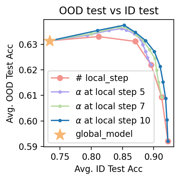
First, we show that taking the interpolation between the personalized model and the global model yields a personalized model with better tradeoffs between the global distribution and the local distribution, where the global distribution is an evenly weighted average of the local objectives. Specifically, we compare the tradeoff curve between in-distribution (ID) and out-of-distribution (OOD) performance of the following methods: Baselines a. pre-train/FedAvg with fine-tuning b. pre-train/FedAvg with origin-regularized fine-tuning, i.e., optimizing the objective \(\min_\theta f_k (\theta)+ WD \times \Vert \theta - \theta_0 \Vert^2\). This penalizes large deviation from the pre-trained model or FedAvg, which tradeoffs between θ^global and θ^per. The WD hyperparameter is to be tuned in practice. c. pre-train/FedAvg with fine-tuning under small LRs. Since using smaller LRs for local fine-tuning yields more refined solutions, we compare fine-tuning with small LRs for more epochs and compare with Soup obtained from larger LR. Specifically,
- LR = 0.0025 ~ fine-tune 10 epochs
- LR = 0.001 ~ fine-tune 25 epochs
- LR = 0.0001 ~ fine-tune 250 epochs Soup pre-train/FedAvg with fine-tuning, followed by performing \(\theta^{\text{per}} \leftarrow \alpha \theta^{\text{per}}+(1-\alpha) \theta^{\text{global}}\)
We try on two datasets:
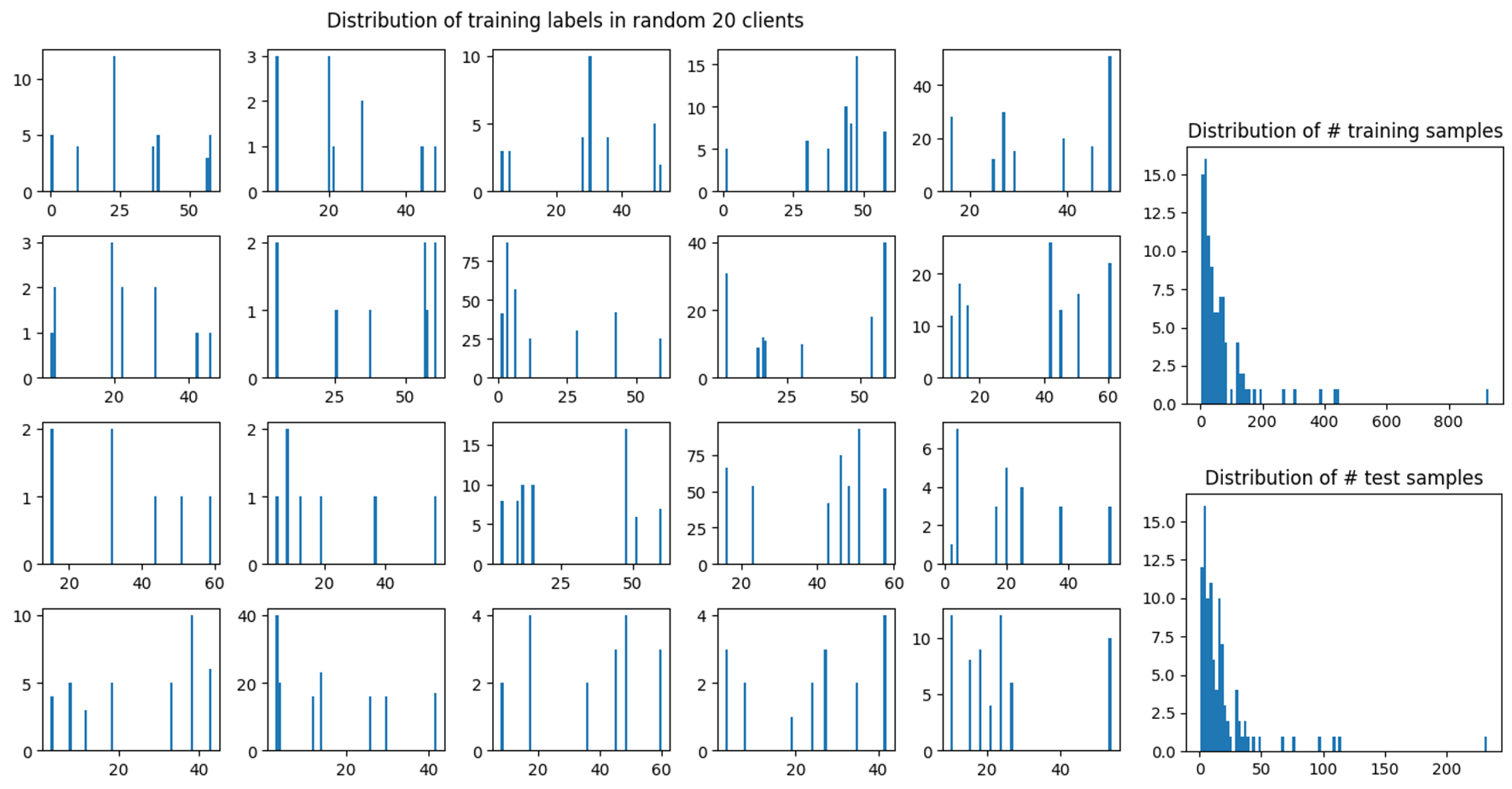
FEMNIST. It is a 62-class classification of the images of hand-written digits/characters. Manual partition by labels to control different levels of heterogeneity. We re-partition the data using the customized parameters, including NUM_USER, num_samples (the number of samples per user), and class_per_user (the number of classes per user). We use the default parameters with the manual partition which gives the following repartition:
We first run FedAvg (as Ditto
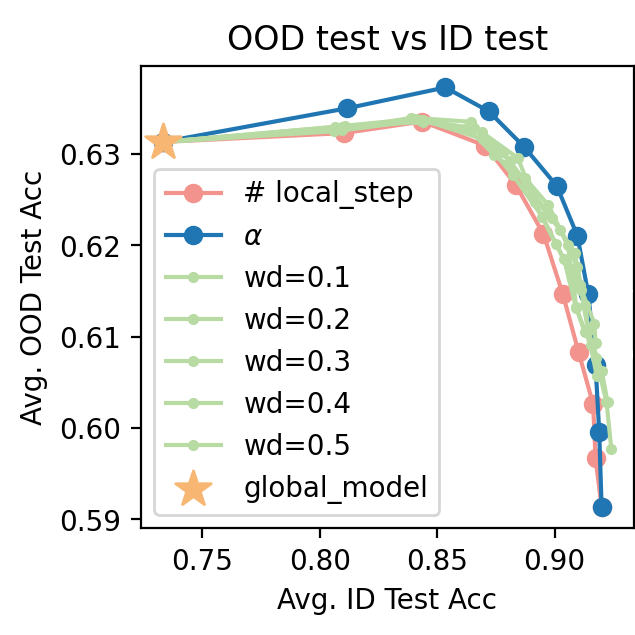
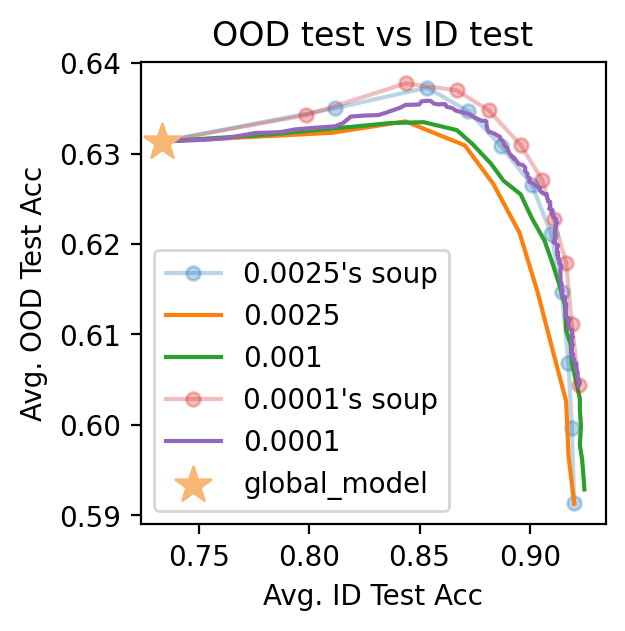
We obtain the takeaway that Soup is always useful:
1. Soup outperforms fine-tuning with regularization.
2. Soup outperforms fine-tuning, including those with smaller LRs: LR=0.0025’s soup has similar performance with LR=0.0001, while <tt>Soup</tt> is 25 times faster.
Google Landmarks. The federated Google landmark dataset is a classification dataset of landmarks images. We use its small gld23k
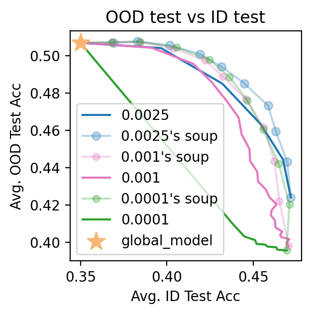
In summary, we observe that
1. Smaller fine-tuning LRs yield better ID-OOD tradeoffs. E.g., LR=0.0001 is similar to the performance of 0.0025’s Soup, though at the cost of being 25 times slower.
2. Soup is always useful: E.g., 0.0001’s soup is better than 0.0001, etc.
Why Effective
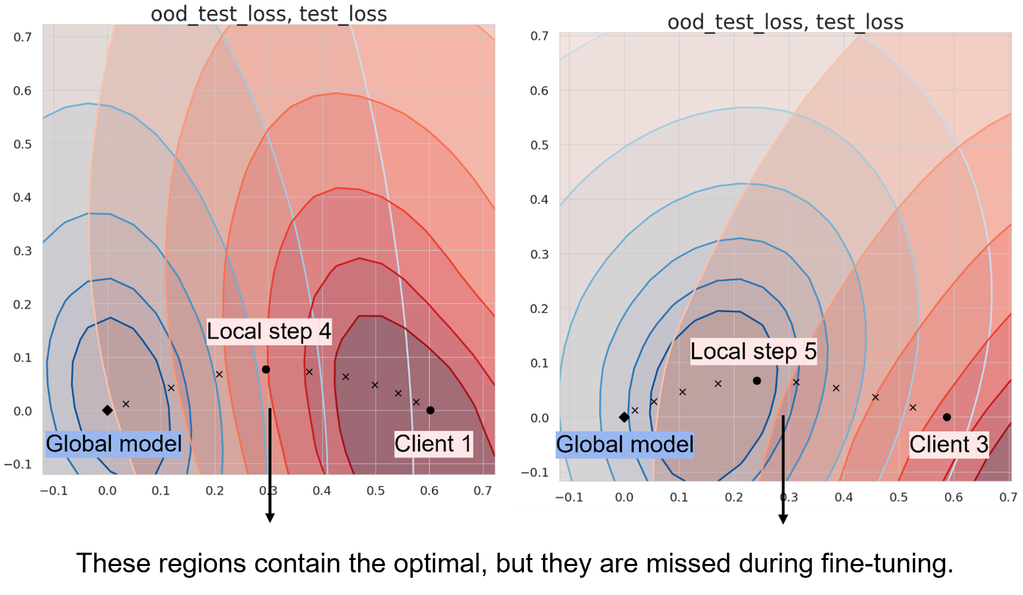
Among the 100 clients, we pick two that benefit from finetuning (client 1 and 3). Next, we visualize why Soup works by plotting the 2D loss landscapes of client 1 and 3’s local test data and global (OOD) test data.
Among all the dimensions of the model, we choose two dimensions by
- The first direction is
step 10 – global model - The second direction is the one in which the intermediate checkpoints have the largest deviation in the direction that is orthogonal to the first direction
For Client 1, we choose basis 1 as Client 1 step 10 – Global and basis 2 as the component of Client 1 step 4 – Global that is orthogonal to basis 1. For Client 3, we choose basis 1 as Client 3 step 10 – Global and basis 2 as the component of Client 3 step 5 – Clobal that is orthogonal to basis 1.
II. Model Exterpolation
Our proposed idea is to extend the weights for aggregation of updates to negative values as a solution to negative transfer. Whether it is in pretrain + finetune or federated scenario, we define \(\lambda\in\mathcal{R}^{K\times K}\) as a transferability matrix that is used as the weights for aggregation by \(W_k^{per}=W_{pre}+\sum_{i=1}^K{\lambda_{ki} \Delta W_i^{ft} }\) where λ indicates the transferability from client \(i\) to client \(k\).
The design is inspired by the fact that (1) when the ground-truth models are linear and (2) each distribution can be represented by a weighted average of all the distributions, then the (same) weighted average of the models are the solutions. This gives us the following problem formulation:
Problem Formulation
Given personalized models \(\{\hat{W}_k \}_{k=1}^K\) that are good approximations of ground-truths \(\{W_k \}_{k=1}^K\). Assume for each client \(k\), \(\exists \{p_k \}_{k=1}^K\) s.t. \(\{(x_i, \tilde{y}_i = \text{argmax}(\sum_{k=1}^K p_k \hat{W}_k x_i))\}_{i=1}^{N_k}\) can better represent client \(k\)’s data distribution. Then \(\tilde{W}_k = \sum_{k=1}^K p_k \hat{W}_k\) is a better personalized model for client \(k\) than \(\hat{W}_k\).
Based on this, we apply it to non-convex models and try two candidates for \(\{p_k \}_{k=1}^K\):
- let \(\lambda_{ki}\) be a reliable distribution similarity metric
- let \(\lambda\) learned by SGD
1. Warmup: Exclude Negative Transfer
Assume that the side information of the distributions of training labels of each client is available, which can work as a natural oracle for the distribution similarity and thus transferability between clients. On FEMNIST manual partition, we have 62 classes, so each client \(i\) has a vector $D(y_i^{tr} )\in [0,1]^{62} $ where \(y_i^{tr}\) is the vector of its training labels. Each index \(j\) at \(D(y_i^{tr})\) represents the proportion of client \(i\) having \(j\)-th class as the label among all its training samples.
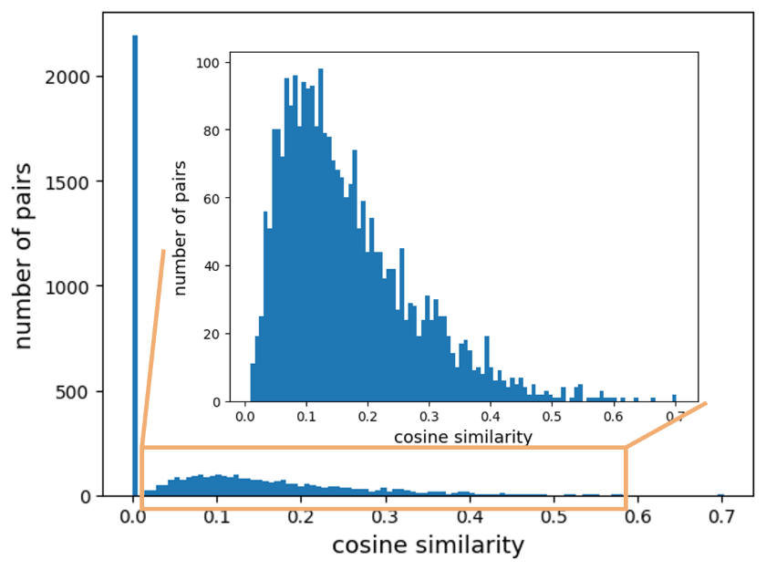
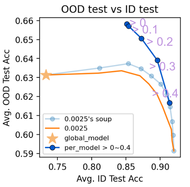
Denoting client \(k\)’s personalized model as \(θ_k^{per}\), we continually update it by \(θ_k^{per}\leftarrow \sum_{i=1}^K \text{CosSim}(D(y_i^{tr} ), D(y_k^{tr} )) \cdot \theta_i^{per}\), which is equivalent to \(\theta_k^{per} \leftarrow \sum_{i=1}^K \mathbb{1} [\text{CosSim}(D(y_i^{tr} ), D(y_k^{tr} ))>0] \cdot \theta_i^{per}\). We have tried 4 more aggregation settings by increasing the cutoff from 0 to 0.1, 0.2, 0.3, and 0.4, respectively. The goal is to show that it is superior to \(\theta_k^{\text{per}}\) under different learning rates as well as the interpolations.
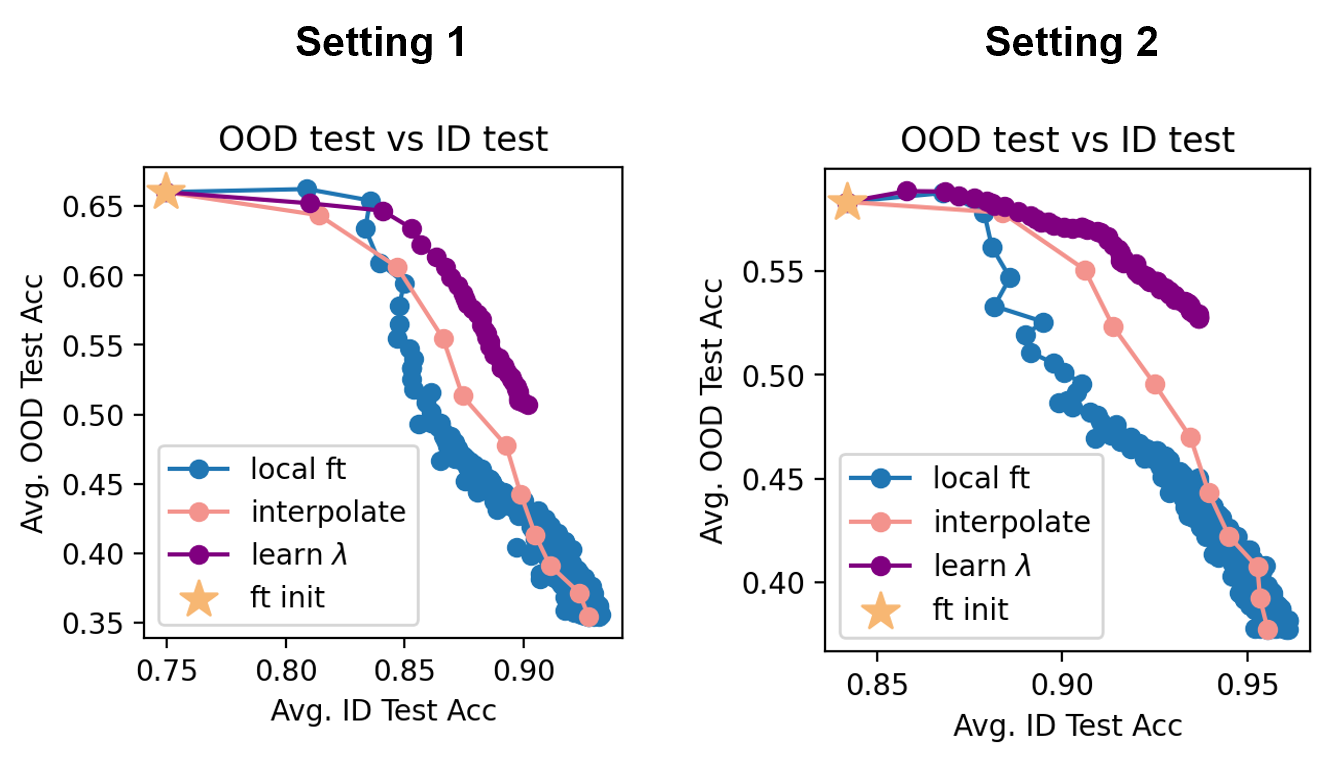
2. Learn \(\lambda\)
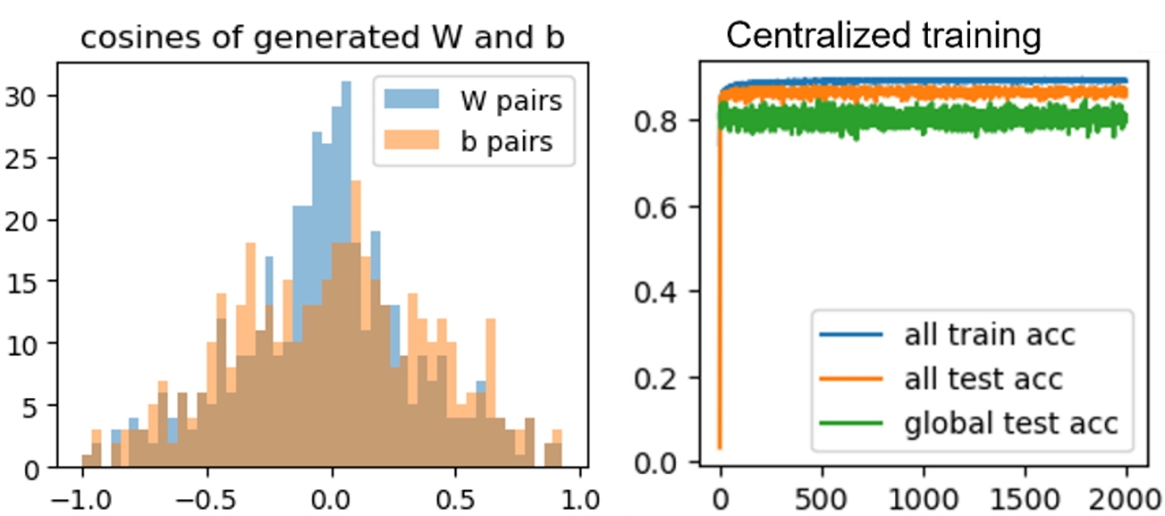
\(\lambda\in\mathbb{R}^{K\times K}\) is a learnable matrix that defines the collaboration relations between distributions. In the following, we run SGD wo momentum to learn \(\lambda\), showing that it outperforms the baselines above. We design and generate three settings of data that is expected to lead to different types of negative transfer.
- 1. Generate $(W_{seed} \in \mathbb{R}^{10\times 60}, b_{seed})$ by having each element of $ W_{seed}\sim\mathcal{N}(0,1), b_{seed}\sim\mathcal{N}(0,1) $, then generate 30 clients' models $\{(W_k, b_k)\}_{k=0}^{29} $ of the same norm but of cosine similarities $\in$ np.linspace(-1, 1, 30) with the seed.
2. Generate ${x_k \in \mathbb{R}^{60}}_{k=0}^{29} $ by $ x_k \sim \mathcal{N}(v_k, \Sigma)$ where $v_k\sim \mathcal{N}(B_k, 1), B_k\sim\mathcal{N}(0, \beta)$ and $\Sigma$ is diagonal with $\Sigma_{j,j} = j^{-1.2}$. Obtain $y_k=\text{argmax} {W_k x_k+b_k}$.
($\beta=1 $)
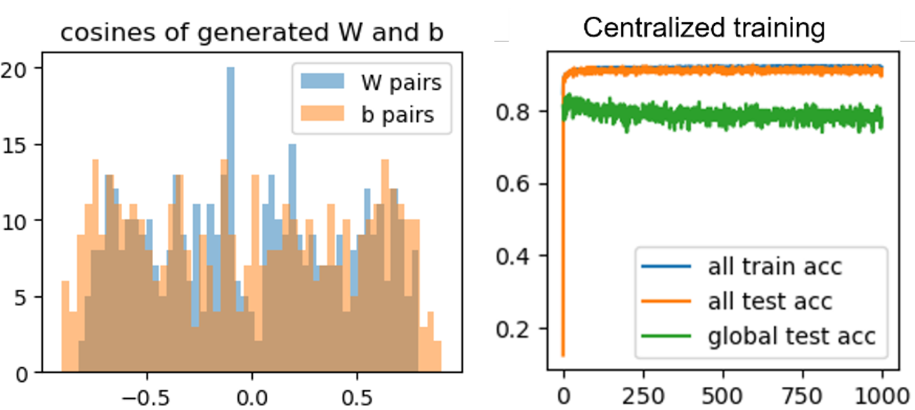
- 1. Generate $\{(W_k, b_k)\}_{k=0}^{29}$ by having each element of $ W_k\sim\mathcal{N}(\mu_k,1), b_k\sim\mathcal{N}(\mu_k,1) $ with $\mu_k\in$np.linear(-alpha,alpha,30).
2. Generate $\{x_k \in \mathbb{R}^{60}\}_{k=0}^{29} $ by $ x_k \sim \mathcal{N}(v_k, \Sigma)$ where $v_k\sim \mathcal{N}(B_k, 1), B_k\sim\mathcal{N}(0, \beta)$ and $\Sigma$ is diagonal with $\Sigma_{j,j} = j^{-1.2}$. Obtain $y_k=\text{argmax} {W_k x_k+b_k}$.
($ \alpha=2, \beta=1 $)